Freezing Rows and Columns in Excel: A Comprehensive Guide

Navigating large Excel spreadsheets can be overwhelming. Scrolling through endless rows and columns makes it difficult to keep track of key data, especially headers. Fortunately, Excel’s freeze panes feature offers a simple solution to this common problem. This guide provides a step-by-step walkthrough on how to freeze rows, columns, or both in Microsoft Excel, along with keyboard shortcuts and comparisons to Google Sheets and Apple Numbers.

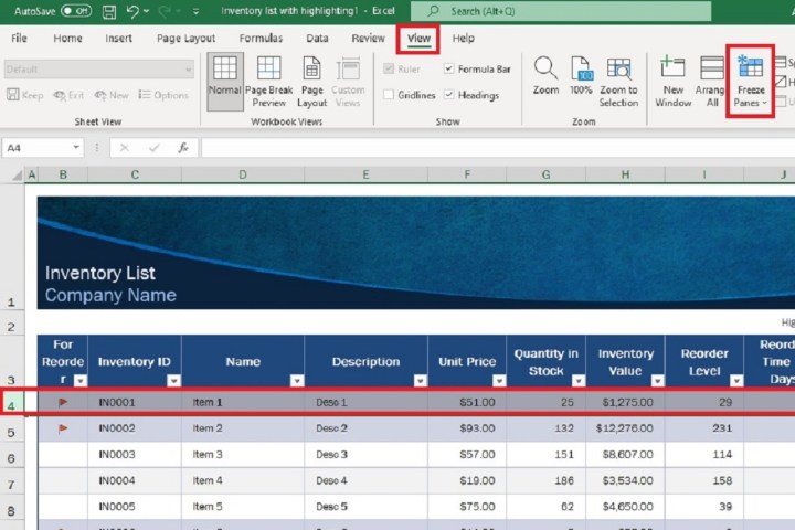An Excel screenshot showing which row to select and the View tab menu for freezing rows.

Freezing Rows in Excel

Freezing rows keeps specific rows visible while scrolling vertically. This is particularly useful for header rows containing labels or categories.

1. Select the Row: Identify the row(s) you want to freeze. Select the row below the last row you want frozen. For example, to freeze rows 1-3, select row 4.

2. Access Freeze Panes: Navigate to the “View” tab in the ribbon menu at the top of the screen.

3. Freeze: Click the “Freeze Panes” dropdown menu and select “Freeze Panes.” To freeze only the top row, choose “Freeze Top Row.”

4. Unfreeze: To unfreeze, return to the “View” tab, click “Freeze Panes,” and select “Unfreeze Panes.”

Freezing Columns in Excel

Similar to freezing rows, freezing columns keeps specific columns visible while scrolling horizontally.

1. Select the Column: Identify the column(s) you wish to freeze. Select the column to the right of the last column you want frozen. To freeze columns A-C, select column D.

2. Access Freeze Panes: Go to the “View” tab in the ribbon.

3. Freeze: Click “Freeze Panes” and select “Freeze Panes.” For freezing only the first column, choose “Freeze First Column.”

4. Unfreeze: Unfreeze by selecting “Freeze Panes” and then “Unfreeze Panes” from the “View” tab. Note: adding a new column within a group of frozen columns will also freeze the new column.

Excel Freeze Panes Keyboard Shortcuts

Streamline your workflow with these handy shortcuts:

1. Freeze Rows and Columns: Alt+W+F+F (press keys sequentially). This freezes rows and columns above and to the left of the active cell.

2. Freeze Top Row: Alt+W+F+R freezes the top row regardless of the active cell.

3. Freeze First Column: Alt+W+F+C freezes the first column, irrespective of the active cell.

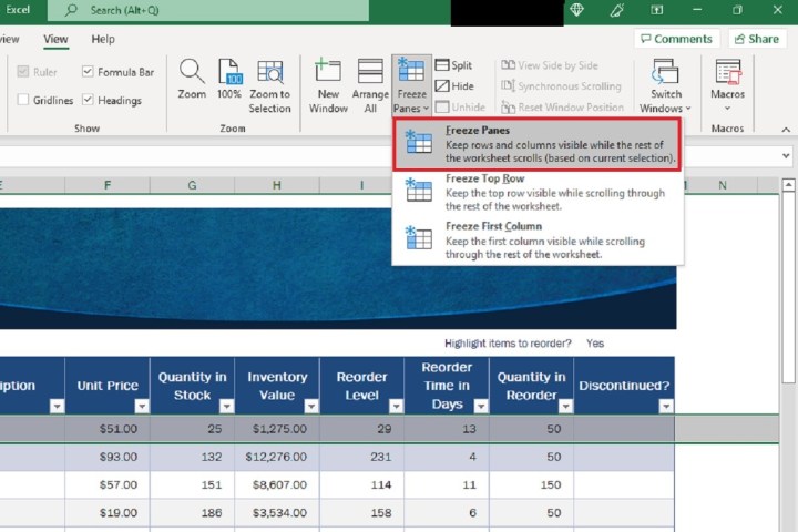An Excel screenshot showing the Freeze Panes drop down menu options.

Freezing Rows and Columns in Google Sheets

Google Sheets offers a similar freeze functionality:

1. Select Row/Column: Choose the row or column you want to freeze.

2. Freeze: Navigate to “View” > “Freeze” in the top menu.

3. Choose Freeze Options: Select the number of rows or columns to freeze. To unfreeze, choose “No rows” or “No columns” under the “Freeze” menu.

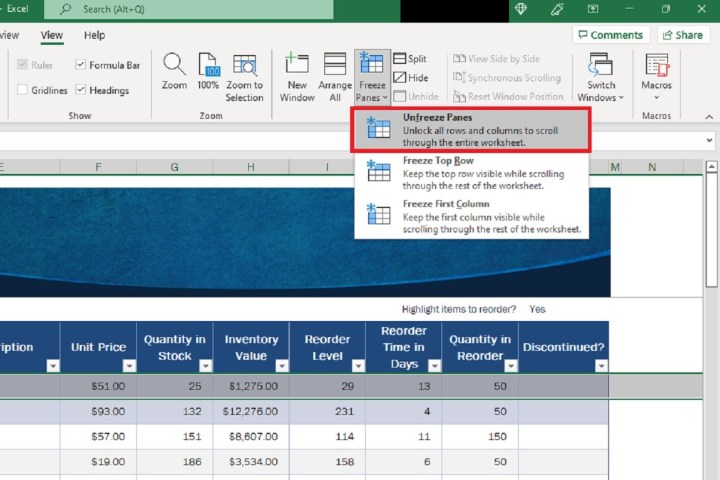An Excel screenshot showing the Unfreeze Panes menu option.

Freezing Rows and Columns in macOS Numbers

Apple Numbers handles freezing differently, focusing on header rows and columns:

1. Select Table: Click anywhere within the table and select “Table” from the top menu.

2. Freeze Headers: Choose “Freeze Header Rows,” “Freeze Header Columns,” or both. You can also adjust the number of header rows or columns to freeze using the “Header Rows” and “Header Columns” options.

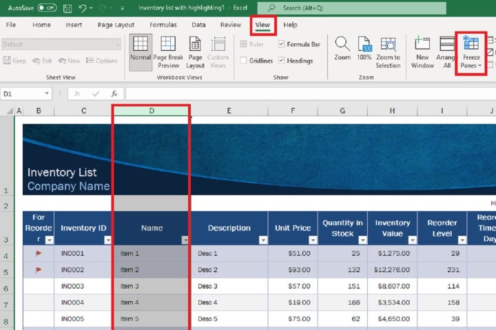An Excel screenshot showing column selection, View tab, and Freeze Panes option.

Conclusion

Freezing rows and columns significantly improves spreadsheet navigation and data analysis. Whether using Excel, Google Sheets, or Numbers, mastering this feature enhances productivity and reduces the risk of data misinterpretation. While freezing panes facilitates efficient scrolling, consider protecting crucial data by learning how to lock cells in Excel for added security.

Google Sheets is open in the Safari browser on a MacBook Air.