Creating drop-down lists in Microsoft Excel is a powerful way to streamline data entry, improve data validation, and enhance the overall user experience. This guide provides a step-by-step approach to creating and customizing drop-down lists in Excel, covering various techniques and best practices.
Using drop-down lists offers several advantages, including saving time compared to manual data entry, minimizing errors by restricting input to predefined options, and ensuring data consistency across spreadsheets. They are ideal for tasks like form creation, data validation, and simplifying complex spreadsheets.
Creating a Drop-Down List by Manual Entry
This method is perfect for beginners and lists that don’t require frequent updates.
Step 1: Select the cell where you want to insert the drop-down list.
Step 2: Navigate to the Data tab and click the Data Validation button (or choose Data Validation from the drop-down menu).
Step 3: In the Data Validation dialog box, select List from the Allow dropdown menu.
Step 4: In the Source field, enter the items for your drop-down list, separated by commas. For example: Option 1, Option 2, Option 3.
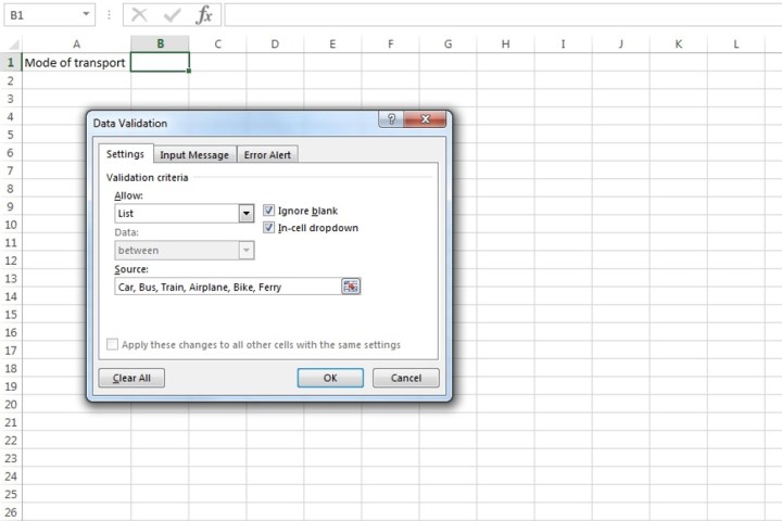 Manually entering data into the Source field for a drop-down list on Microsoft Excel.Image used with permission by copyright holder
Step 5: Click OK. Your drop-down list is now active in the selected cell.
Creating a Drop-Down List from a Cell Range
This method is more versatile and suitable for larger lists and dynamic data.
Step 1: Enter the data for your drop-down list in a separate column or even a separate spreadsheet. This keeps your main worksheet organized.
Step 2: Populate the column with your list items, each in its own cell.
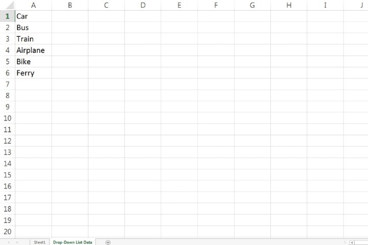 Inputting entries for a drop-down list on Microsoft Excel.Image used with permission by copyright holder
Step 3: Select the cell where you want the drop-down list to appear.
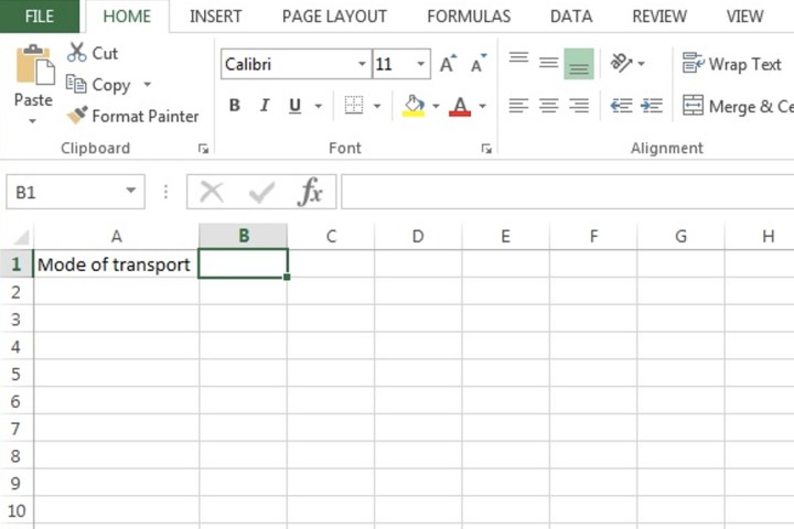 Selecting the cell for a drop-down list on Microsoft Excel.Image used with permission by copyright holder
Step 4: Go to the Data tab and select Data Validation.
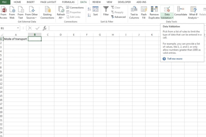 The Data Validation button on Microsoft Excel.Image used with permission by copyright holder
Step 5: In the Data Validation dialog, choose List from the Allow menu. Click the arrow icon next to the Source field.
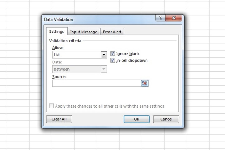 The List option within the Allow menu on Microsoft Excel.Image used with permission by copyright holder
Step 6: Select the range of cells containing your list items.
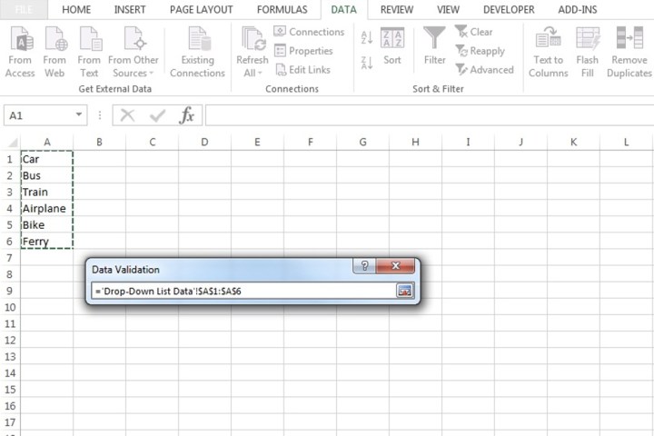 Selecting a range of cells for a drop-down list on Microsoft Excel.Image used with permission by copyright holder
Step 7: Click the arrow icon in the Data Validation dialog again. The Source field now displays the selected range. Click OK.
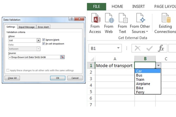 The Source bar that includes the range of cells required for a drop-down list.Image used with permission by copyright holder
Adding an Input Message
Provide helpful guidance to users by displaying a message when the cell with the drop-down list is selected.
Step 1: Select the cell containing the drop-down list and open the Data Validation dialog.
Step 2: Go to the Input Message tab. Enter a title and a descriptive message (up to 225 characters).
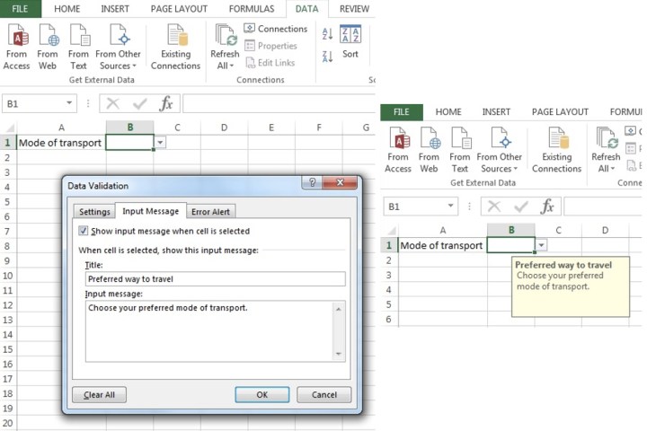 Displaying a message for a drop-down list on Microsoft Excel.Image used with permission by copyright holder
Step 3: Click OK.
Displaying an Error Alert
Guide users with error alerts for invalid entries.
Step 1: Select the drop-down list cell and open the Data Validation dialog. Choose the Error Alert tab.
Step 2: Check the Show error alert after invalid data is entered box. Enter a title and message. Select a style (Stop, Warning, or Information).
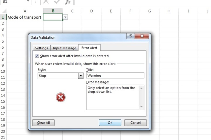 Entering the relevant data for displaying an error alert for a drop-down list on Microsoft Excel.Image used with permission by copyright holder
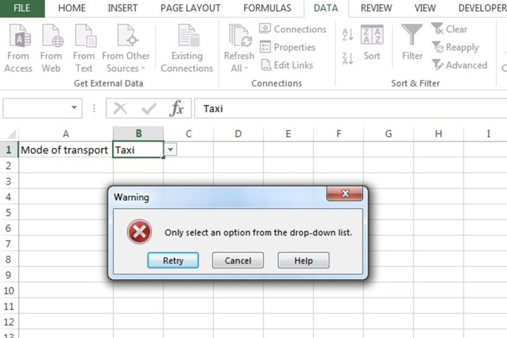 Displaying an error alert for a drop-down list on Microsoft Excel.Image used with permission by copyright holder
Step 3: Click OK.
Protecting Your Drop-Down List
Prevent unauthorized changes to the source data of your drop-down list.
Step 1: Select the cells containing the source data.
Step 2: Go to the Home tab, click the small arrow in the Alignment section to open the Format Cells dialog. On the Protection tab, check the Locked box and click OK.
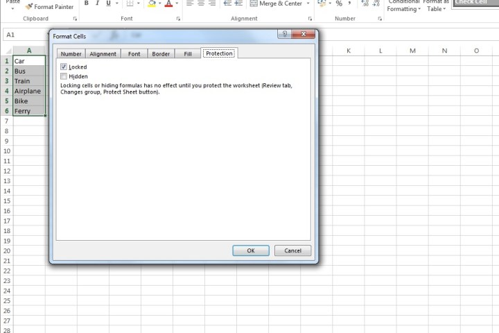 Locked option checked.Image used with permission by copyright holder
Step 3: Go to the Review tab and select Protect Sheet or Protect Workbook. Configure the protection settings as needed and click OK.
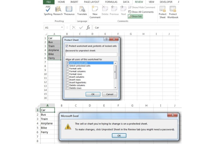 The Protect Worksheet option for locking cells on Microsoft Excel.Image used with permission by copyright holder
Conclusion
By mastering these techniques, you can leverage the power of drop-down lists to create more efficient, user-friendly, and error-free Excel spreadsheets. From basic list creation to advanced customization and protection, this guide provides the tools you need to enhance your Excel workflow.


