The CONCATENATE function in Microsoft Excel, while perhaps less renowned than stalwarts like IF and VLOOKUP, offers a powerful way to merge data from multiple cells into a single cell or column. This functionality proves invaluable for various tasks, such as combining revenue and profit data for a given month. This guide provides a comprehensive walkthrough of using CONCATENATE in Excel, covering different scenarios and customization options.
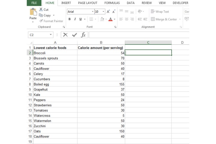 Using the concatenate formula in Excel to merge data.Image used with permission by copyright holder
CONCATENATE takes data from two or more cells and merges it into a third. It’s important to distinguish this from the “Merge & Center” feature, which primarily affects formatting. CONCATENATE, on the other hand, is a data manipulation tool. Let’s delve into its practical application.
Combining Data from Two Columns
Here’s a step-by-step guide to using CONCATENATE with two columns:
-
Select the Destination Cell: Choose the cell where you want the combined data to appear. This can be any cell within your spreadsheet. For this example, we’ll use the column adjacent to the two columns being combined.
-
Enter the Formula: To combine cells A2 and B2, enter the following formula:
=CONCATENATE(A2,B2). This is the most basic form of the function.
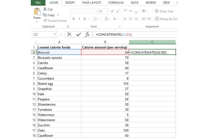 Entering the concatenate formula into a cell in Excel.Image used with permission by copyright holder
- Confirm the Formula: Press Enter to execute the formula. The data from the specified cells will be merged into the destination cell.
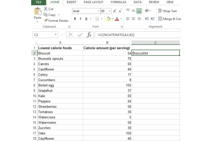 How a cell looks after inputting the concatenate formula in Excel.Image used with permission by copyright holder
- Customize the Output: The basic formula merges the data directly, which might not always be ideal. To add a space between the combined data, use the following formula:
=CONCATENATE(A2," ",B2). You can insert any character or string within the quotation marks. For example, to separate the data with an equal sign and spaces, use:=CONCATENATE(A2," = ",B2).
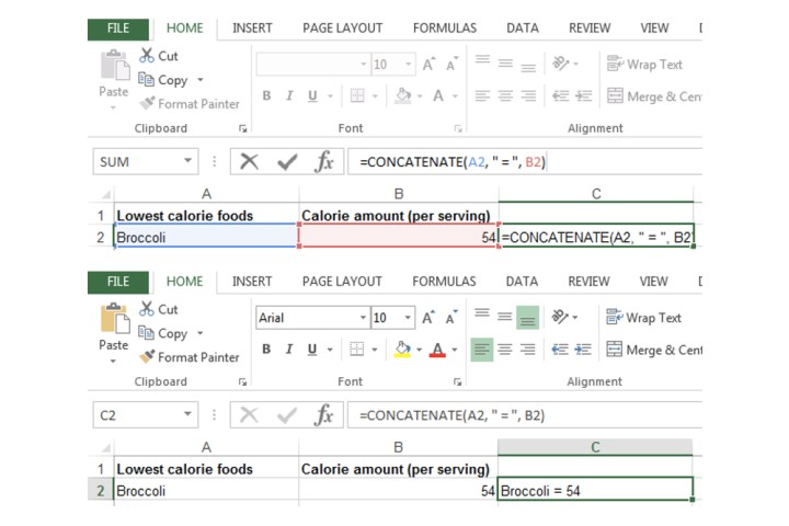 Adding a space and equal sign within a concatenate formula in Excel.Image used with permission by copyright holder
- Format the Cell: Use standard Excel formatting tools to enhance the appearance of the combined data. You can adjust font size, style (bold, italic), alignment, and more.
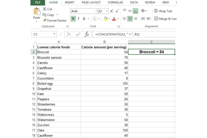 Applying further customization to a cell where the concatenate function has been applied.Image used with permission by copyright holder
Concatenating Three or More Columns
CONCATENATE isn’t limited to two columns. To combine three columns (A2, B2, and C2), use the formula: =CONCATENATE(A2,B2,C2). Remember to adjust the column letters as needed.
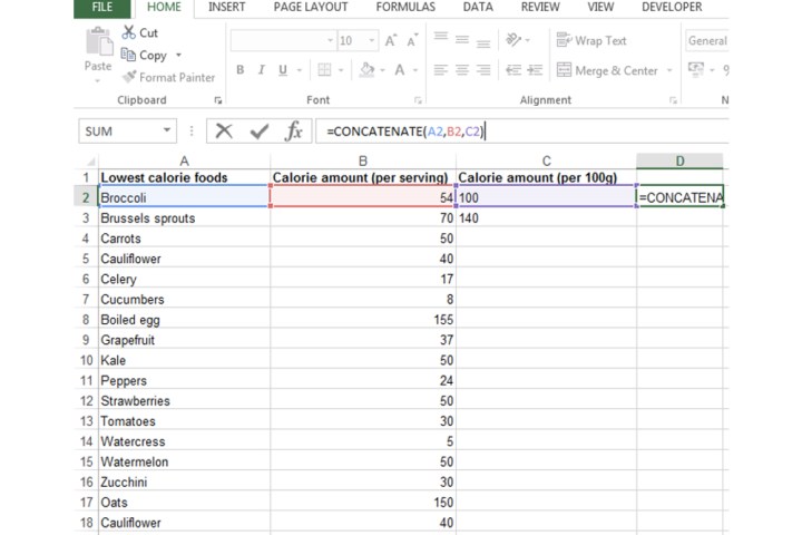 The concatenate formula for combining three columns in Excel.Image used with permission by copyright holder
To apply this formula to an entire column, simply drag the fill handle (the small square at the bottom right of the cell) down to the desired range.
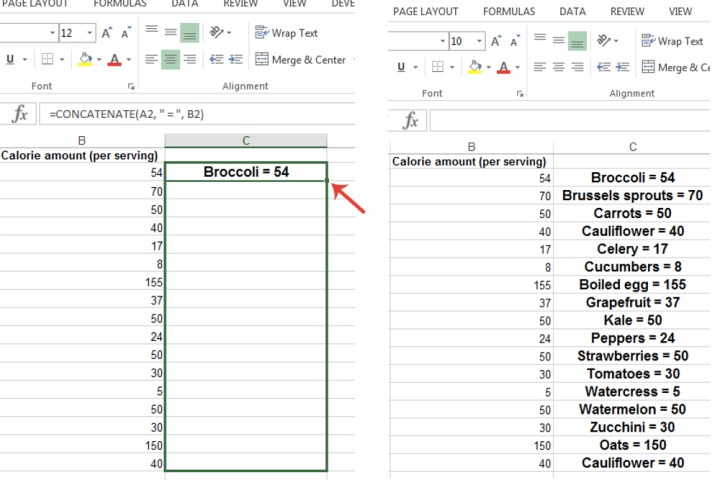 Applying the concatenate formula by dragging a cell in Excel.Image used with permission by copyright holder
Concatenating Without the Formula
Excel offers a shorthand method for concatenation using the ampersand (&) operator. For example, =A2&B2 achieves the same result as =CONCATENATE(A2,B2). This can be a more concise way to combine data.
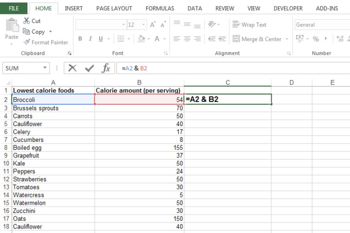 Applying the concatenate function in Excel without the formula.Image used with permission by copyright holder
This guide has provided a comprehensive overview of the CONCATENATE function in Excel, enabling you to effectively merge data and streamline your spreadsheet workflows. For more Excel tips and tutorials, explore our resources on creating graphs and alphabetizing data.


